In this post we will consider a simple financial calculator to see the effect of compounding interest, and also to estimate the number of years a particular sum of funds is able to last through retirement.

The code will prompt the user to consider two scenarios, each with a starting amount, and the annual increment. This is followed by the input of the interest rate used for calculating the appreciation and the duration involved. The calculation is such that the annual interest is first added onto the initial sum, before the annual increment set by the user is added on.

Let us consider the block of code below.

Line 1 imports the pandas module. This will be the only module that is required for this Python example.
Line 3 to 11 creates the variables, taking in the user input as floats, for the starting amount and annual increment for the two scenarios respectively.
Line 13 creates the variable for the user to input the interest rate to be used for the calculation. Note that a 4% interest rate should be entered as a value of 1.04. Likewise, Line 15 creates the variable for the user to input the duration to be considered.

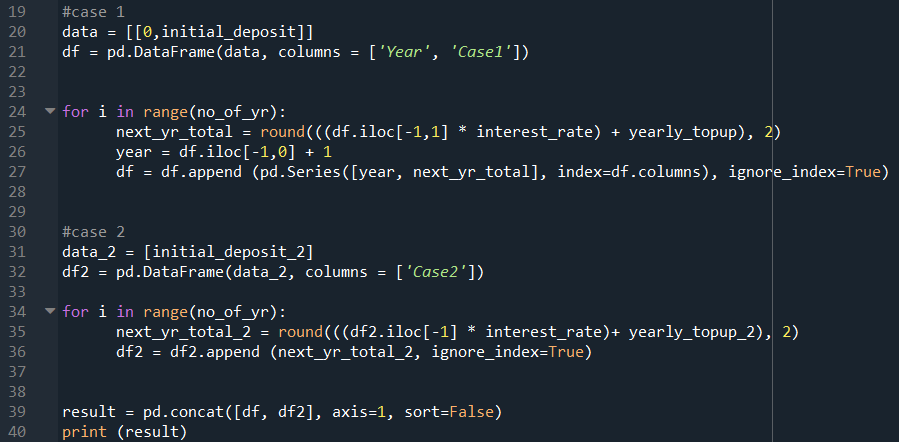
Line 20 stores the user inputs from the first scenario (Case 1) as an array. Line 21 creates a new dataframe to store this initial data, with the stated column headers.
Line 24 to 27 uses a for loop to add the annual interest to the principal sum, followed by the stated annual increment. This means that it will be looking at the last row of the previous iteration to do the calculations. The value is then rounded to two decimal place. The number of loops, or iterations, is determined by the duration to be considered.
Line 31 to 36 repeats the above process with the second scenario (Case 2), storing the calculation in another dataframe.
Line 39 then concatenates the two dataframes column-wise, and prints out the combined data in the IPython console for the user’s reference.

Line 43 to 44 then print out the final amount at the end of the specified duration in the IPython console for the user’s reference as well.
Using the matplotlib function in pandas module, a line graph could be plotted using Line 48.
Line 49 set the y-axis limit to have a minimum value to zero (the purpose of this line will be described later…)
Line 51 and 52 has been commented out as shown above. You can choose to use these two lines to export the graphs as a picture.

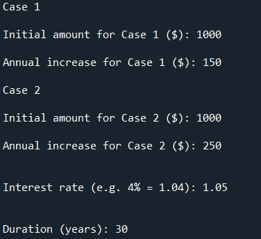
Let’s consider an example where the user wants to calculate a savings plan, beginning with the same initial amount, but chooses a different annual increment. Interest rate is set at 5% for a duration of 30 years.

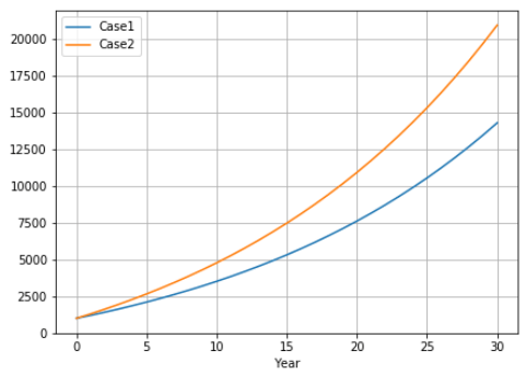
The graph generated shows the different growth that would be obtained:

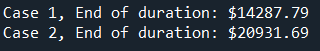
A dataframe with the actual amount each year will be displayed in the IPython console (not sshown here). The final amount for each case is also output in the IPython console as shown below:

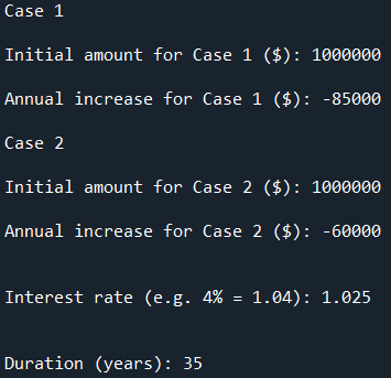
This same code can also be used to consider the duration a particular sum could last for retirement given different annual drawdown amount. Consider an initial amount of $1 M, with the drawdown amount as shown; in this case a negative number is input. The remaining amount can still earn some interest, in this case 2.5%. We shall see if this can last us for 35 years. Note that the calculation is such that the interest at the end of the first year is added before the drawdown occurs from the second year.

The graph generated is shown below:

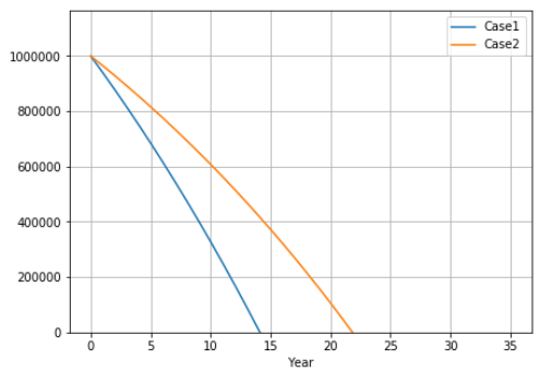
It seems that neither of the two cases can last for 35 years. Case 1 would only last for slightly less than 15 years, while Case 2 for about 22 years.

Based on the way we calculate the amount for each year, there is not much meaning to the number once the value becomes negative. Thus the graph is truncated at a y-axis value of $0, as dictated by Line 49 in the code.

Is there any way to make the above codes more concise and elegant? Feel free to comment.