This post will be looking at using the k-Nearest Neighbour (kNN) algorithm for a classification problem. Suppose there is a new data point that is required to be classified into one of the known categories that comprises the data. This algorithm will look at the k closest points (where k is an integer specified by the user) to the data of interest using distance measures such as Euclidean distance, for example. Each of these k objects votes for their category and the category with the most votes is taken as the prediction.

For this example, the Leaf Data Set from the UCI Machine Learning Repository will be used.

Reference
https://archive.ics.uci.edu/ml/datasets/Leaf (Accessed on 01 Feb 2020)
“The data included can be used for research and educational purposes only. All publications using this dataset should cite the following paper:
‘Evaluation of Features for Leaf Discrimination’, Pedro F.B. Silva, Andre R.S. Marcal, Rubim M. Almeida da Silva (2013). Springer Lecture Notes in Computer Science, Vol. 7950, 197-204.“

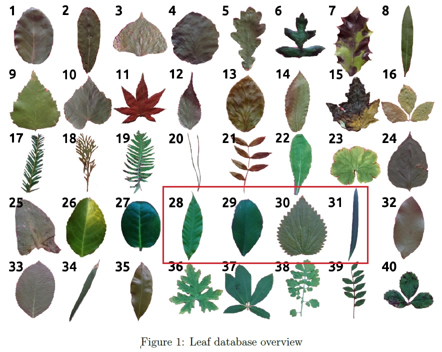
Based on the documentation provided, this leaf database consists of 40 different leaf species as shown below and for the purpose of this illustration, kNN classification will be applied to species number 28 to 31 (so chosen as they should present a simple and straightforward classification problem).

Let us consider the block of code below for applying the kNN algorithm for this classification problem. The code shown would not start from Line 1 or have continuous Line numbering as with previous post, as some comments/notes present in the code has been omitted for simplicity sake.

We begin with some basic data preparation.

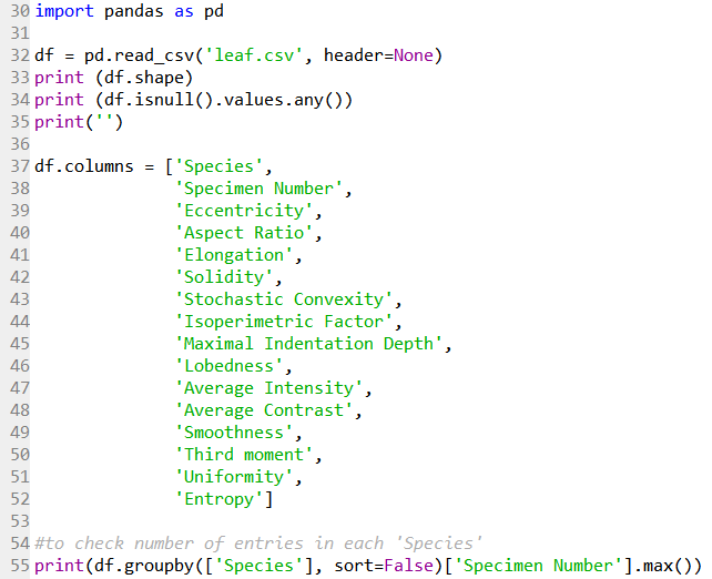
Line 30 imports the Pandas module for data handling. Line 32 reads the .csv file downloaded from the repository as a Pandas dataframe. Line 33 returns the size of the data as (340 rows, 16 columns). Line 34 returns False, meaning there are no NaN values in the data.

Line 37 to 52 then label the column heading with the labels as described in the dataset documentation.

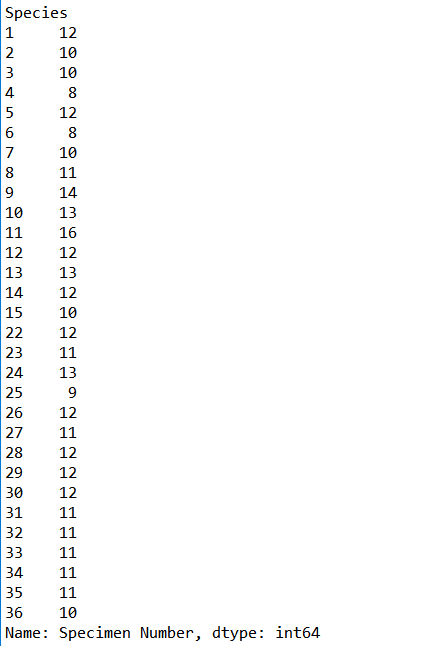
Line 55 then returns the number of specimen samples (right column), as an integer dtype, in each Species category (left column). It is evident that the data for Species category 37 to 40 is missing from the .csv file, but not really a problem for now as the data of interest is not affected.

The data subset containing species number 28 to 31 will be selected and visualised to provide some insights into the data.

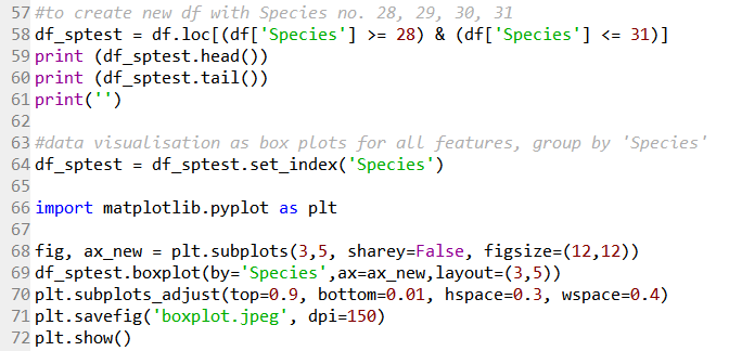
Line 58 creates a new dataframe with only data from species number 28 to 31 that should be a matrix of (47 rows, 16 columns). Line 59 to 60 give a quick check of the first five and last five rows of the data.

Line 64 set the ‘Species’ column data as the index.

Line 66 imports the matplotlib module for subsequent graph generation for data visualisation. Line 68 and 69 creates a 3×5 matrix of boxplot subplots to visualise the various features (column data), with each subplot having their own axis range. Line 70 formats the spacing between each subplot, and the overall plot. Line 71 saves the boxplots as a .jpeg file as shown below.

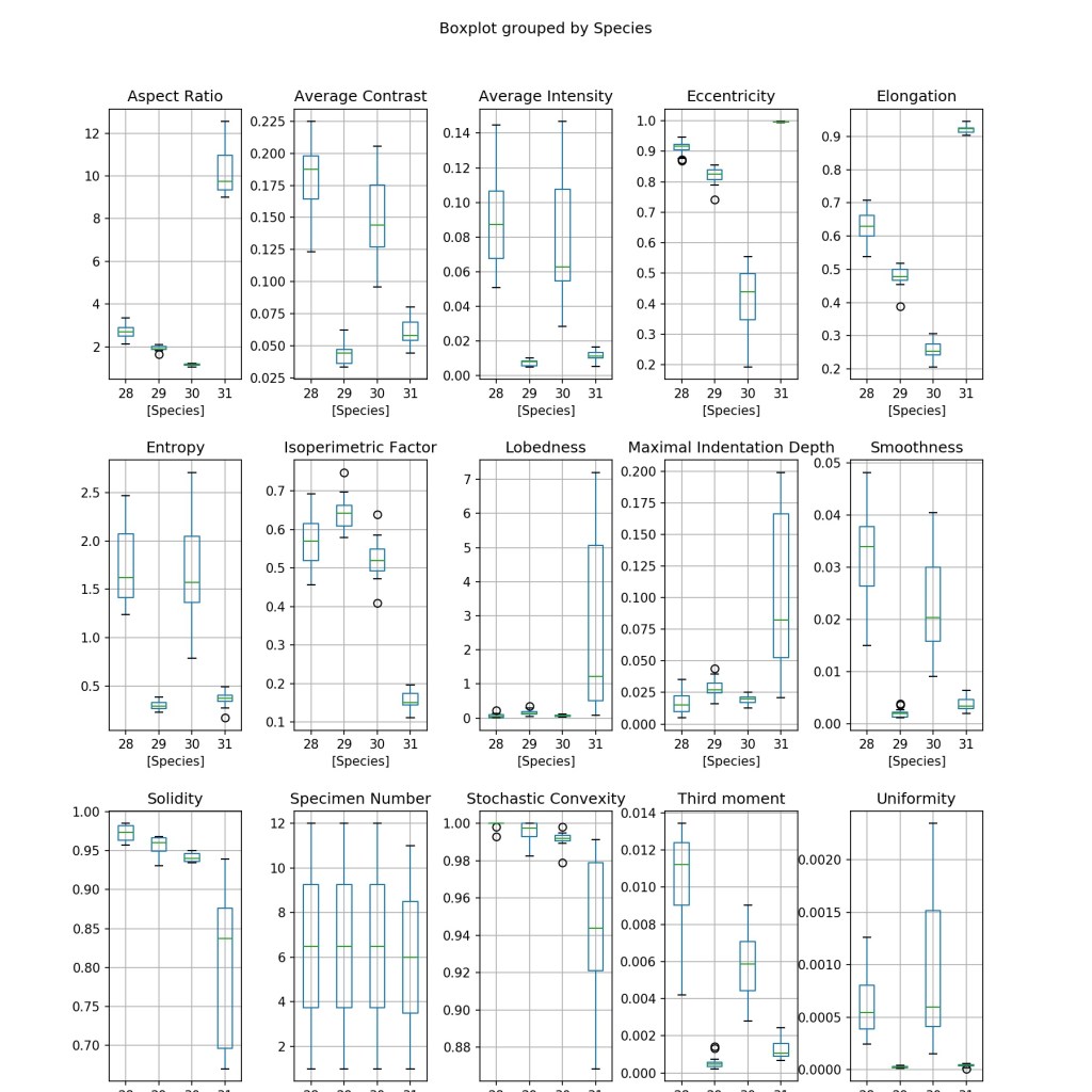
It is clear that some features are useful for distinguishing all the four species (e.g. Elongation) due to the distinct values of each species, while some might be useful for only identifying a particular species (e.g. Lobedness).

Line 74 to 76 imports the required functions from the sklearn module to perform the kNN classification.

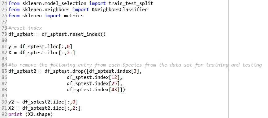
Before we carry on, the index is reset via the code in Line 79, as the ‘Species’ column data was previously set for the purpose of the boxplots. The data is then separated into target variables (i.e. the ‘Species’ info), and the feature variables (i.e. all other columns except the ‘Specimen Number’ column) in Line 81 and 82.

Line 85 to 88 removes a sample from each of the ‘Species’ category to be used later on. Line 90 and 91 then creates a new target and feature variable set to be used with the kNN algorithm later. The feature variable X2 would have a shape of (43 rows, 14 columns).

In Line 94, the train_test_split function splits the X2 feature variables into a training set, and a test set comprising of 20% of the data. A value of random_state = 50 is use for reproducibility purposes.

The question now being what should be the value of k to be used in our kNN model?

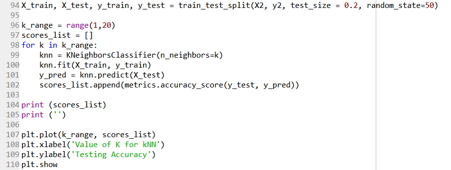
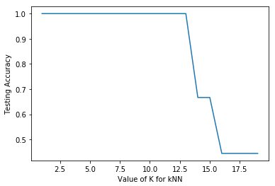
Line 96 to 102 used a for loop to iterate the process of obtaining the accuracy score of the kNN model with a range of k values from 1 to 19. This can be considered as a form of hyperparameter tuning with regard to the n_neighbors parameter. Line 107 to 110 then plot the results as a graph as shown below.

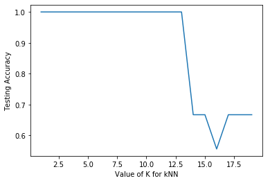
The plot shows that the accuracy is 100% up to a n_neighbor value of 12, and then decreases significantly thereafter. It is expected that with larger value of n_neighbor, more data points are being considered leading to poorer ability to distinguish between the Species categories.

First a n_neighbor value of 5 will be used in the model, and the four samples that were excluded earlier will be used to validate the model.

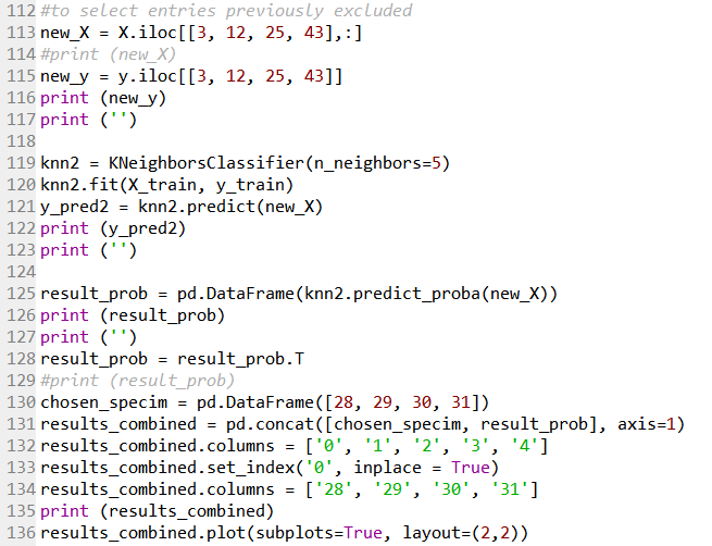
Line 113 and 115 creates a new target and feature variable of the four samples that was excluded previously. Line 119 to 122 uses the kNN model with n_neighbor value of 5 to predict the target of these four samples.

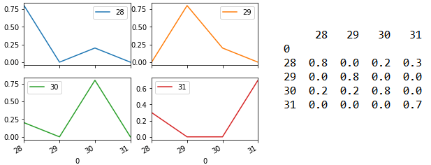
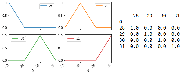
Line 125 returns prediction probability as an array. For each sample, the probability of it having the different target (i.e. Species category 28/29/30/31) will be shown. Line 128 to 135 then formats this array into the matrix shown on the right side below. Line 136 output this as four subplots shown on the left below. The model is able to predict each of the four samples with 100% accuracy.

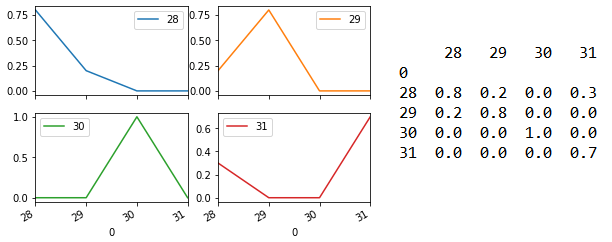
What if a n_neighbor value of 10 is used instead?
Based on the graph above, the accuracy only drops with a n_neighbor value greater than 12.

Changing Line 119 to n_neighbor = 10 shows that the prediction performance has now decreased although the model still predicts the correct species category.

However, using an odd integer for the n_neighbor value is a common practice as it helps to prevent the possibility of a statistical stalemate (i.e. there are equal numbers from two different categories).

Moving on, an observation of the earlier boxplots again shows that the following features have a distribution that is distinct for each of the four species:
– Average contrast
– Average Intensity
– Eccentricity
– Elongation
– Smoothness
– Third moment

Thus, let see what changes to the results are observed should the kNN model be applied with just these six features.

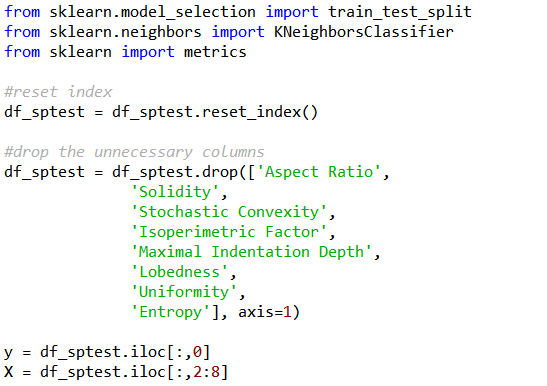
To remove the unnecessary feature columns, the code for the section marked “#drop the unnecessary columns” could be inserted between Line 79 and 81 previously. As the number of feature column is lesser, the range of columns to be sliced by the feature variable X has to be amended accordingly.

The accuracy score of the kNN model with a range of k values from 1 to 19 is still very much similar.

The following shows the results for n_neighbors = 5.

While the following shows the results for n_neighbors = 10.

Perhaps it is not surprising that application of the model with just six features is comparable to the model with all fourteen features, given that the six chosen features have values that are distinct to each species.

In this case, the more relevant features could be singled out rather easily. For more complicated cases, other methods might be used to determine feature importance.

Is there any way to make the above codes more concise and elegant? Feel free to comment.

The StandardScaler function from sklearn.preprocessing was used to normalise all features used in a separate study not shown in this post, and it was found that the model generated is not as good as the one shown here.

Also, such a post might be better illustrated using Jupyter Notebook, but that is a topic for another time...