One common analysis a chemist does in a laboratory is the use of high performance liquid chromatography (HPLC) to determine the concentration of a particular analyte.

After the method development is complete, a typical workflow for sample analysis is as follows:
i) Measurement of the peak areas of various known concentration of the calibration standard.
ii) Plot the calibration curve in a spreadsheet.
iii) Analyse the required sample to obtain the peak area.
iv) Transfer data to spreadsheet, and calculating the corresponding analyte concentration using the best fit line obtained from the calibration curve.

Nowadays, the software accompanying the HPLC equipment would have an in-built function to expedite this process. However, let’s see how it can be automated using a Python code.

Suppose the peak areas of various known standard solutions are obtained and saved in a file Calib.csv as shown below.

A set of four samples were also analysed, and their corresponding peak areas are obtained and saved in a file Expt1.csv as shown below.

How then could the sample concentration of each of the four samples in Expt1.csv be obtained without manually transferring the data to a spreadsheet and setting up the cells with their corresponding formulae?

Let us consider the block of code below.

Line 1 and 2 import the numpy and pandas modules required to handle the data. Line 3 imports the matplotlib module to plot the calibration curve. Line 4 imports the mean function from the statistics module to be used in the calculation of the best fit line.

Line 9 to 11 read the Calib.csv file and prints them to the Python console.
Line 12 to 15 then go through the Calib.csv file to identify the columns with the concentration and area data, as well as the values of the lowest and highest concentration values used for the calibration curve.

Line 18 to 38 first defines the function of obtaining the gradient m and y-intercept b of the best fit line (using least square regression), calculate the R-squared value of the best fit line, followed by printing out the data to the Python console. Line 24 to 25 could also be used, by removing the comment character ‘#’, to change the number of decimal places of the various parameters of the best fit line (currently set as four decimal places).

Line 41 to 42 use the values from the least square regression to generate the data points for the best fit line. Line 44 plots the peak areas obtained from the calibration samples as a scatter plot, while Line 45 plots the best fit line as a blue line. Line 47 to 50 formats the plot with the plot title, axes labels, and display both the line and scatter plot as a single graph in the Python console.

Line 52 to 55 calculate the corresponding concentration of the four samples in Expt1.csv and append this result as a new column in the pandas dataframe. Line 57 to 58 then save the results as a new file (Results Expt1.csv).

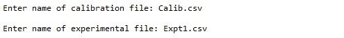
Once the code is run, the user would be prompted to input the name of the calibration file, and the experimental file containing the data to be analysed. (A try-except error handling could also be added in the code to capture potential typographical error by the user.)

Thereafter, Calib.csv would be read, followed by the printout of the details of the calibration curve, a plot of the calibration curve, and the calculated concentration of each of the samples.

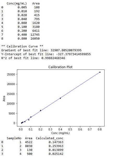
A new file (Results Expt1.csv) would then be created in the same folder, containing the calculated concentrations appended as a new column as shown below.

Note – The above code requires the .csv files to be in the same folder as the .py file, whereas in reality, the HPLC results would be saved in folders typically assigned to their project name and date of analysis. In addition, the data used would not be in the format as shown in Expt1.csv, thus the code would need to be changed to read the comma separated values accordingly.

However, the above code offers a short example of using Python to automate this process, and could be easily modified to access the required files in their respective folders.

Is there any way to make the above codes more concise and elegant? Feel free to comment.

You can also check out the corresponding video on Youtube:
https://youtu.be/4JS69AMWRGo
There is a section towards the end of the video showing how the code executes in a Python IDE.