This post will be a little (just a little…) intensive on the physical chemistry side of things as I explore the other functions of the Python Programming Language, using an example on reaction kinetics.
Let’s consider the following reaction scheme showing the elementary reactions, where the starting material A gets converted to B with a rate of k1, but decomposes further to C with a rate of k2. As such, it is advantageous to stop the reaction at a particular time where the amount of B is at its maximum.

The rate law of each step can be defined as follows (Equation (i) to (iii)).

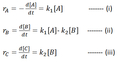
The concentrations of A and B could be determined at various time, t, using equations (iv) and (v) by integrating the equations above. (Let’s not dwell too much on the mathematics to obtain equation (v)…)
By mass balance (i.e. C can only come from B, and B from A and nothing else), the concentrations of the A, B and C must sum to the initial concentration of A, [A]0 (equation (vi)).

References for equations from “The Chemical Reactor from Laboratory to Industrial Plant”, Elio Santacesaria and Riccardo Tesser, Springer Nature Switzerland AG 2018, Chapter 4, pp. 244-245.

With equations (iv) to (vi) in hand, a reaction profile of concentration vs time could be obtained for all the components present in this reaction. Let us consider the block of code below.

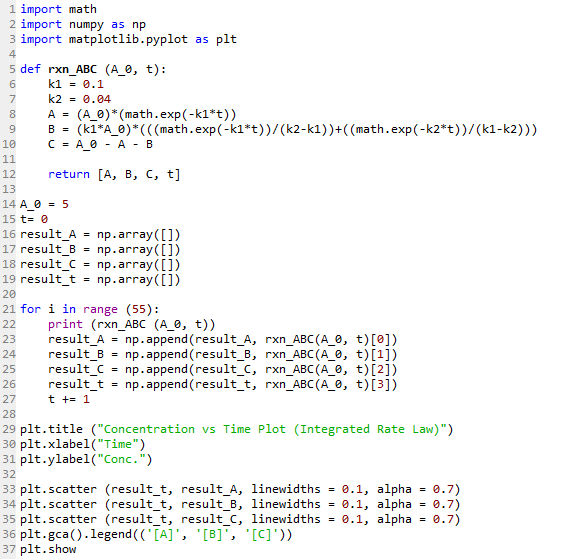
Line 1 imports the math module required for using the exponential e function in the equations later. Line 2 imports the numpy module while Line 3 imports the matplotlib module to generate the plot at the end.
Line 5 to 12 defines the function rxn_ABC that will be used to calculate the concentrations of the three components with respect to time. Here, the rate constants k1 and k2 are defined arbitrarily as 0.1/s and 0.04/s respectively.
Line 8 to 10 is simply equations (iv) to (vi) shown previously, with Line 12 returning the results whenever the function rxn_ABC is called.
Line 14 to 15 set the initial condition, with t = 0 and initial concentration of A, [A]0, at 5 M.
Line 16 to 19 creates an empty array for each of the variables A, B, C and t.
Line 21 to 27 uses a for loop to calculate the concentrations of A, B and C at the various time points, up to t = 55, and appending each result to the respective array created earlier.
Line 29 to 37 then creates the plot of the concentrations of A, B and C versus t as shown below. Each series is plotted using the array data of the component versus time.

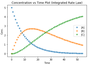
As seen from the plot above, the concentration of B reaches a maximum before it decreases as time progresses. Thus, the reaction is required to be stopped at that point to prevent more B from decomposing and lowering its yield.

Alternatively, if you are an organic chemist like myself, with the unfortunate lack in mathematical capabilities, there is a package in Python that can help with solving the differential equations.

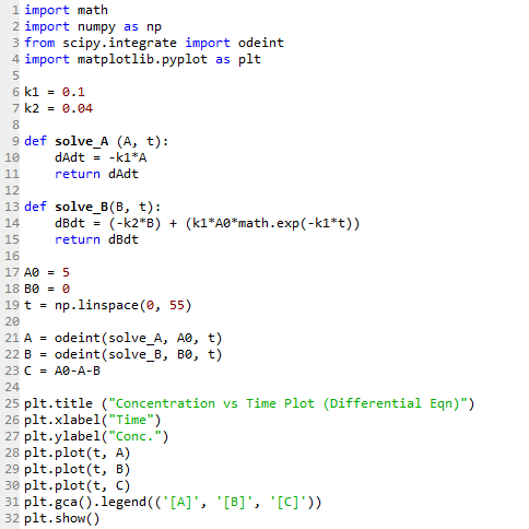
The same Python packages are used as before, with the addition of the odeint function from scipy as imported in Line 3.
Line 6 to 7 defines the same constants k1 and k2 being used.
Each differential equations is defined as a separate function. Line 9 to 11 defines the function to describe equation (i); Line 13 to 15 for equation (ii), with [A] being substituted by equation (i).
Line 17 to 18 defines the initial state with [A]0 = 5 M and no B present.
Line 19 creates the array for the time values, from 0 to 55.

Solving the differential equations is as simple as Line 21 to 22.
Line 23 is the mass balance equation (vi) used to calculate the concentration of C.
Line 25 to 32 then creates the plot of the concentrations of A, B and C versus t as shown below.

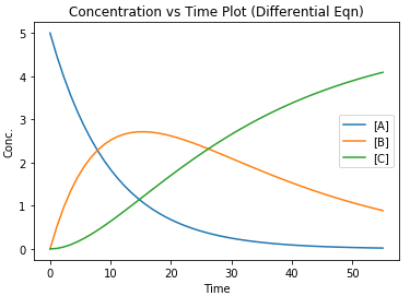
No surprises here – The concentration versus time plot obtained using the two methods described above pretty much gives the same results.

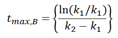
The time with the maximum concentration of B can be calculated using the equation shown below, which is obtained when d[B]/dt = 0.

Is there any way to make the above codes more concise and elegant? Feel free to comment.